
Dimensions give context to measures. Typical analysis includes pivot tables and pivot graphs. These pivot on one or more dimension columns used for analysis—these columns are called attributes in DW and OLAP terminology.
Columns with unique values identify rows. These columns are keys. In a data warehouse,
you need keys just like you need them in an LOB database. Keys uniquely identify entities. Therefore, keys are the second type of columns in a dimension.
Pivoting makes no sense if an attribute’s values are continuous, or if an attribute has too
many distinct values. Imagine how a pivot table would look if it had 1,000 columns, or how a pivot graph would look with 1,000 bars. For pivoting, discrete attributes with a small number of distinct values is most appropriate. A bar chart with more than 10 bars becomes difficult to comprehend. Continuous columns or columns with unique values, such as keys, are not appropriate for analyses.
If you have a continuous column and you would like to use it in analyses as a pivoting attribute, you should discretize it. Discretizing means grouping or binning values to a few discrete groups. If you are using OLAP cubes, SSAS can help you. SSAS can discretize continuous attributes. However, automatic discretization is usually worse than discretization from a business perspective. Age and income are typical attributes that should be discretized from a business perspective. One year makes a big difference when you are 15 years old, and much less when you are 55 years old. When you discretize age, you should use narrower ranges for younger people and wider ranges for older people (these are used for Graph type pivoting).
A customer typically has an address, a phone number, and an email address. You do not analyze data on these columns. You do not need them for pivoting. However, you often need information such as the customer’s address on a report. If that data is not present in a DW, you will need to get it from an LOB database, probably with a distributed query. It is much simpler to store this data in your data warehouse. In addition, queries that use this data perform better, because the queries do not have to include data from LOB databases. Columns used in reports as labels only, not for pivoting, are called member properties.
In addition to the types of dimension columns already defined for identifying, naming,
pivoting, and labeling on a report, you can have columns for lineage information,
A dimension may contain the following types of columns:
■■ Keys Used to identify entities
■■ Name columns Used for human names of entities
■■ Attributes Used for pivoting in analyses
■■ Member properties Used for labels in a report
■■ Lineage columns Used for auditing, and never exposed to end users
Hierarchies
Figure 1-9 shows the DimCustomer dimension of the AdventureWorksDW2012 sample database.
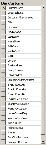
In the figure, the following columns are attributes (columns used for pivoting):
■■ BirthDate (after calculating age and discretizing the age)
■■ MaritalStatus
■■ Gender
■■ YearlyIncome (after discretizing)
■■ TotalChildren
■■ NumberChildrenAtHome
■■ EnglishEducation (other education columns are for translations)
■■ EnglishOccupation (other occupation columns are for translations)
■■ HouseOwnerFlag
■■ NumberCarsOwned
■■ CommuteDistance
All these attributes are unrelated. Pivoting on MaritalStatus, for example, is unrelated to
pivoting on YearlyIncome. None of these columns have any functional dependency between them, and there is no natural drill-down path through these attributes. Now look at the Dim- Date columns, as shown in Figure 1-10.

Some attributes of the DimDate edimension include the following (not in the order shown in the figure):
■■ FullDateAlternateKey (denotes a date in date format)
■■ EnglishMonthName
■■ CalendarQuarter
■■ CalendarSemester
■■ CalendarYear
You will immediately notice that these attributes are connected. There is a functional dependency among them, so they break third normal form. They form a hierarchy. Hierarchies are particularly useful for pivoting and OLAP analyses—they provide a natural drill-down path. You perform divide-and-conquer analyses through hierarchies.
Hierarchies have levels. When drilling down, you move from a parent level to a child level. For example, a calendar drill-down path in the DimDate dimension goes through the following levels: CalendarYear ➝ CalendarSemester ➝ CalendarQuarter ➝ EnglishMonthName ➝ FullDateAlternateKey
At each level, you have members. For example, the members of the month level are, of course, January, February, March, April, May, June, July, August, September, October, November, and December. In DW and OLAP jargon, rows on the leaf level—the actual dimension rows—are called members. This is why dimension columns used in reports for labels are called member properties.
In a Snowflake schema, lookup tables show you levels of hierarchies. In a Star schema, you need to extract natural hierarchies from the names and content of columns. Nevertheless, because drilling down through natural hierarchies is so useful and welcomed by end users, you should use them as much as possible.
Slowly Changing Dimensions
There is one common problem with dimensions in a data warehouse: the data in the dimension changes over time. This is usually not a problem in an OLTP application; when a piece of data changes, you just update it. However, in a DW, you have to maintain history. The question that arises is how to maintain it. Do you want to update only the changed data, as in an OLTP application, and pretend that the value was always the last value, or do you want to maintain both the first and intermediate values? This problem is known in DW jargon as the Slowly Changing Dimension (SCD) problem.
The problem is best explained in an example. Table 1-1 shows original source OLTP data
for a customer.
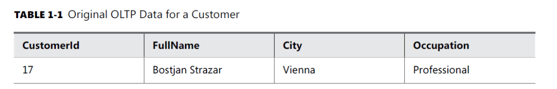
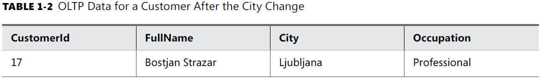
The customer lives in Vienna, Austria, and is a professional. Now imagine that the customer moves to Ljubljana, Slovenia. In an OLTP database, you would just update the City column, resulting in the values shown in Table 1-2.
If you create a report, all the historical sales for this customer are now attributed to the
city of Ljubljana, and (on a higher level) to Slovenia. The fact that this customer contributed to sales in Vienna and in Austria in the past would have disappeared.
In a DW, you can have the same data as in an OLTP database. You could use the same key,
such as the business key, for your Customer dimension. You could update the City column when you get a change notification from the OLTP system, and thus overwrite the history.
Type 1 SCD : Type 1 means overwriting the history for an attribute and for all higher levels of hierarchies to which that attribute belongs.
The problem here would rise that you want to store the historical data . What if we want transactions of the same customer when he did in Vienna ? The solution to this problem would be to add a surrogate key (DW key ).
Type 2 SCD : When you implement Type 2 SCD, for the sake of simpler querying, you typically also add a flag to denote which row is current for a dimension member. Alternatively, you could add two columns showing the interval of validity of a value.

You could have a mixture of Type 1 and Type 2 changes in a single dimension. For example, in Table 1-3, you might want to maintain the history for the City column but overwrite the history for the Occupation column. That raises yet another issue. When you want to update the Occupation column, you may find that there are two (and maybe more) rows for the same customer. The question is, do you want to update the last row only, or all the rows? Table 1-4 shows a version that updates the last (current) row only, whereas Table 1-5 shows all of the rows being updated.

Fact Table Column Types
Fact tables are collections of measurements associated with a specific business process. You store measurements in columns. Logically, this type of column is called a measure. Measures are the essence of a fact table. They are usually numeric and can be aggregated. They store values that are of interest to the business, such as sales amount, order quantity, and discount amount.
All foreign keys together usually uniquely identify each row and can be used as a composite primary key.
For example, suppose you start building a sales fact table from an order details table in a source system, and then add foreign keys that pertain to the order as a whole from the Order Header table in the source system. Tables 1-7, 1-8, and 1-9 illustrate an example of such a design process.
Table 1-7 shows a simplified example of an Orders Header source table. The OrderId
column is the primary key for this table. The CustomerId column is a foreign key from the Customers table. The OrderDate column is not a foreign key in the source table; however, it becomes a foreign key in the DW fact table, for the relationship with the explicit date dimension. Note, however, that foreign keys in a fact table can—and usually are—replaced with DW surrogate keys of DW dimensions.
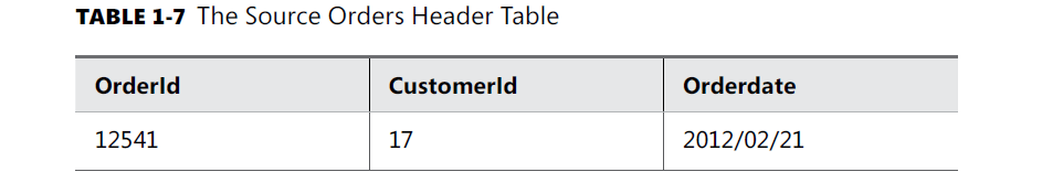
Table 1-8 shows the source Order Details table. The primary key of this table is a composite one and consists of the OrderId and LineItemId columns. In addition, the Source Order Details table has the ProductId foreign key column. The Quantity column is the measure .

Table 1-9 shows the Sales Fact table created from the Orders Header and Order Details
source tables. The Order Details table was the primary source for this fact table. The OrderId, LineItemId, and Quantity columns are simply transferred from the source Order Details table.
The ProductId column from the source Order Details table is replaced with a surrogate DW ProductKey column. The CustomerId and OrderDate columns take the source Orders Header table; these columns pertain to orders, not order details. However, in the fact table, they are replaced with the surrogate DW keys CustomerKey and OrderDateKey.
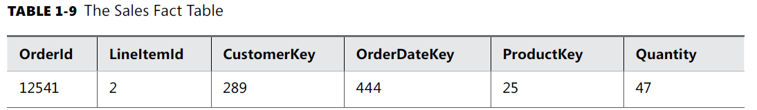
You do not need the OrderId and LineItemId columns in this sales fact table. For analyses, you could create a composite primary key from the CustomerKey, OrderDateKey, and Product- Key columns.
Additivity of Measures
Additivity of measures is not exactly a data warehouse design problem. However, you should consider which aggregate functions you will use in reports for which measures, and which aggregate functions you will use when aggregating over which dimension.
The simplest types of measures are those that can be aggregated with the SUM aggregate
function across all dimensions, such as amounts or quantities. For example, if sales for product A were $200.00 and sales for product B were $150.00, then the total of the sales was $350.00.
If yesterday’s sales were $100.00 and sales for the day before yesterday were $130.00, then the total sales amounted to $230.00. Measures that can be summarized across all dimensions are called additive measures.
Some measures are not additive over any dimension. Examples include prices and percentages, such as a discount percentage. Typically, you use the AVERAGE aggregate function for such measures, or you do not aggregate them at all. Such measures are called non-additive measures.
For some measures, you can use SUM aggregate functions over all dimensions but time.
Some examples include levels and balances. Such measures are called semi-additive measures.
For example, if customer A has $2,000.00 in a bank account, and customer B has $3,000.00, together they have $5,000.00. However, if customer A had $5,000.00 in an account yesterday but has only $2,000.00 today, then customer A obviously does not have $7,000.00 altogether. You should take care how you aggregate such measures in a report. For time measures, you can calculate average value or use the last value as the aggregate.
Quick Question :
■■ You are designing an accounting system. Your measures are debit, credit, and
balance. What is the additivity of each measure?
Answer: Debit and credit are additive measure while balance is semi additive measure.
Summary :
■■ Fact tables include measures, foreign keys, and possibly an additional primary key and lineage columns.
■■ Measures can be additive(fixed total sum of sales ) , non-additive(price changes or percentage changes ), or semi-additive(credit and debit in account) 32
.
