Git has three main states that your files can reside in: committed, modified, and staged.
Committed means that the data is safely stored in your local database.
Modified means that you have changed the file but have not committed it to your database yet.
Staged means that you have marked a modified file in its current version to go into your next commit snapshot.
The Git directory is where Git stores the metadata and object database for your project. This is the most important part of Git, and it is what is copied when you clone a repository from another computer.
The working directory is a single checkout of one version of the project. These files are pulled out of the compressed database in the Git directory and placed on disk for you to use or modify.
The staging area is a file, generally contained in your Git directory, that stores information about what will go into your next commit.
The basic Git workflow goes something like this:
You modify files in your working directory.
You stage the files, adding snapshots of them to your staging area.
You do a commit, which takes the files as they are in the staging area and stores that snapshot permanently to your Git directory.
If a particular version of a file is in the Git directory, it’s considered committed. If it’s modified but has been added to the staging area, it is staged. And if it was changed since it was checked out but has not been staged, it is modified.
Initializing a Repository in an Existing Directory
$ git init
This creates a new subdirectory named .git that contains all your necessary repository files—a Git repository skeleton. At this point, nothing in your project is tracked yet.
Cloning an Existing Repository
If you want to get a copy of an existing Git repository—for example, a project you’d like to contribute to—the command you need is git clone. If you’re familiar with other VCS systems such as Subversion, you’ll notice that the command is “clone” and not “checkout.” This is an important distinction—instead of getting just a working copy, Git receives a full copy of nearly all data that the server has. Every version of every file for the history of the project is pulled down by default when you run git clone. In fact, if your server disk gets corrupted, you can often use nearly any of the clones on any client to set the server back to the state it was in when it was cloned
You clone a repository with git clone [url]. For example, if you want to clone the Git linkable library called libgit2, you can do so like this:
$ git clone https://github.com/libgit2/libgit2

That creates a directory named libgit2, initializes a .git directory inside it, pulls down all the data for that repository, and checks out a working copy of the latest version. If you go into the new libgit2 directory, you’ll see the project files in there, ready to be worked on or used.
Recording Changes to the Repository
You have a bona fide Git repository and a checkout or working copy of the files for that project. You need to make some changes and commit snapshots of those changes into your repository each time the project reaches a state you want to record.
Remember that each file in your working directory can be in one of two states: tracked or untracked. Tracked files are files that were in the last snapshot; they can be unmodified, modified, or staged. Untracked files are everything else—any files in your working directory that were not in your last snapshot and are not in your staging area. When you first clone a repository, all your files will be tracked and unmodified because you just checked them out and haven’t edited anything.
As you edit files, Git sees them as modified, because you’ve changed them since your last commit.
An object is an Entity, for example: car, house , person, time etc. Object can be tangible or intangible.
Lets consider a car (tangible) which is our object . An object has an attribute, behaviour and has a unique Id.
Car has attribute (color, model) , behaviour ( accelerate, brake the car, change gear) and has a unique registration number.
Now , lets take an intangible object example: Time. A time can have attributes like: Year, month, day. A time can have its behaviour set, like set the Year, set the Month, set the day and it can have a unique identifier : Date of birth, date of joining the college, date of creation.
Information hiding:
Some characteristics of object are:
Information is stored within an object.
It is hidden from outside world.
It can only be manipulated by the object itself.
Example: An object called Alex who is a person and he is our object model, the outside world or any other person cannot know his name by seeing him or interacting with him. We cannot also know his exact age until he lets us know. We can get his name and age only when he wants us to let us know. So, we cannot access his name and age directly but we can ask him to tell his name.
Another example is contact numbers stored on a mobile phone. A mobile phone is an object. It is hiding phone numbers inside it. If i want to get a number starting from letter ‘S’ then i have to ask or access the phone to get me the list of numbers starting from ‘S’.
So information hiding simplifies the process. An object Alex enquires from object phone to tell him the numbers starting from ‘S’. So in short, Alex’s information like age or name is hidden until he tells you or he gives access to his details and you cannot access the phone numbers until you get access to the phone itself and perform the operations.
2. Encapsulation:
State and behaviour of an object are tightly coupled. You can perceive an object whose name is Alex and age is 36. You do not know how he has stored that information in his brain, when you ask him , he performs that operation and then lets you know his name and age. You do not know in which part of the brain he has that information and how he got it.
A phone has stored a phone number in digital format and knows how to convert in human readable format. A user does know how data is stored and how it is converted to human readable format.
3. Object has an interface:
An object encapsulates data and behaviour. So how objects interact with each other ? Each object provides an interface (operations).
So lets say , an object whose name is Alex. You ask Alex in english , what is your name ? So he will tell you his name. If you ask him any other thing like where are you going or what is your plan , you will never get his name. So in simple terms the only interface which Alex has allowed to get exposed to you or outer world is by asking what is your name. Any other way you try to get his name , you will not get it.
Another example can be: an object car , whose interface can be : Steer wheels, change gear, accelerate, apply brakes.
If you want to speed up the car you have to accelerate. If you want to change the direction of the car you will use its interface steer wheels, if you have to stop the car you have to apply the brakes interface, you cannot stop the car if you try to use any other interface!
Abstraction:
Abstraction is a way to cope with complexity and reduce the complexity .
Principle of abstraction: Capture those details about an object that are relevant to that perspective.
For example: Alex is a student of PhD in a school and teaches some undergrad student courses. He might be having attributes like studentId, badge no, age, year,CGPA, Employee Id, designation, salary.
So it seems he is a student as well as a teacher in the school. There can be other more perspectives to the object Alex, like his sports playing perspectice like his score, his match date, his jersey no. There can be his medical perspectives like his height, age, blood group, his vaccination dates etc. These are different perspectives related to Alex. To make things simple in OOP, we only relate the object to its perspective and this way we make things simple.
Lets take the example we highlighted in bold , where Alex is a PhD student as well as a teacher. There are two perspectives one as a student (studentId, badge no, age, year, CGPA) and one as a teacher(EmployeeId, designation, salary).
Similarly , Alex’s behaviour as a student can be: study, play sports, give exams.
Alex’s behaviour as a teacher can be deliver lecture, prepare exam, teach and take exam.
Lets take another example : A car with a driver’s perspective and engineer’s perspective.
Driver’s perspective: A car has 4 doors, white color, a steering wheel, good seats.
Engineer’s perspective: Structure of car, engine, number of rods, wheel type etc .
So each perspective is separate and making them separate will reduce complexity.
Classes:
In OOP Model: Some of the Objects exhibit identical characteristics ( information structure and behaviour).
We say they belong to the same class.
For example: There are 15 students in a class room. They exhibit almost same behaviour, they take notes, sit on a chair and give the exam. So we can instantiate each student as an object with identical characteristics.
Take another example of a wooden stamp which has a government seal. When you stamp it , it creates a different object but the characteristic is same, the government seal.
So, take an example: A student class , there are three students , Alex who studies maths, Katherine who studies chemistry and Jack studies Physics. We created three objects here as an instance of student class.
In Python, every piece of data is represented as an instance of some class. A class provides a set of behaviors in the form of member functions (also known as methods), with implementations that are common to all instances of that class. A class also serves as a blueprint for its instances, effectively determining the way that state information for each instance is represented in the form of attributes (also known as fields, instance variables, or data members).
Inheritance:
A child inherits characteristics of his parents.
Besides that a child may also have its own unique characteristics.
If class B inherits from class A, then class B will have all characteristics (attributes and behaviour) of class A . A parent class is called Base class and child class is called derived class.
Consider a Parent class Person having its child classes student, teacher and doctor.
A parent class shape having child classes circle, triangle and line.
A person parent class has (name,age, eat( ), walk( ) ) has a derived class student (class, year, study( ), give exam( ) ) and a class teacher (employeeId, designation, teach( ), take exam( ) ).
Generalization in Inheritance:
The derived class inherit general characteristics.
A teacher and a student both eat and walk. So we can put these characteristics in a base class called person.
Person(name,age, gender, walk( ), eat( ) ) .
Student (program,year, give exam( ), study( ) ) and Teacher( designation, employee Id, take exam( ), teach( ) ).
Student is a person. Teacher is a person.
2. Subtyping( Extension) :
Sub-typing means that derived class is behaviourally compatible with base class. Behaviourally compatible means that base class can be replaced by derived class.
3. Speciaization(Restriction):
Specialization means that derived class is behaviourally incompatible with base class.And it means that base class cannot always be replaced by derived class.
Suppose a base class called Person has a derived class Adult. Person <– Adult , now if we add a restriction in adult class that age < 18 then it cannot be an adult , so Person class then cannot be replaced by Adult class.
Another example is base class called Integer Set (add(element) ) which has derived class called Natural Set( add(element) ).
Integer Set (add element( ) ) <– Natural Set (add element( ) ).
Consider an integer Set class which includes negative, zero and positive numbers. Now lets look at Natural set ,which can only include 0,1,2,3 and so on.. It cannot include negative numbers. So a Natural Set class is a specialized class of Integer Set class.
4. Overriding:
A derived class may override a default behaviour from its parent class but may exhibit totally new behaviour or new implementation. This is called overriding.
The reasons for overriding can be:
Provide a new behaviour specific to the derived class
Restricting default behaviour.
Extend the default behaviour.
Improve performance.
For example : In Integer Set class we use add(element) to add two variables but in Natural Set we can use to add 5 elements.
Overriding concept is under inheritance in OO modeling not outside it.
Abstract Classes
An abstract class implements abstract concept.
Main purpose is to be inherited by other classes.
Cannot be instantiated.
Promotes re use.
In the person and student,teacher , doctor classes example, person class can be an abstract class. Firstly the abstract class are mostly at top of the hierarchy so it can be inherited. A person class can be an abstract class because in real life for example : we say he is a doctor , he is a student , she is a teacher, not he is a person, she is a person.
Take another example of a shape class which has a derived class called circle, line, triangle. We do not say it is a shape when we see a circle or a triangle in real life. We say it is a circle or a triangle.
That is why we keep abstract class at the top because it exhibits general , common concept like : shape, person, vehicle.
Rather than the classes from which we can create objects from are called concrete classes. Like teacher , doctor, student from Person class . Car, truck , cycle from vehicle class. So we instantiate object from a concrete class .
Multiple Inheritance:
A class inherited from multiple classes is said to have multiple inheritance. For example : If i have to create a mermaid i have to inherit properties of a human and a fish. So in OO model a mermaid class will be made from human class and a fish class.
Association:
Alex drives a car. It can have 1….* association. Alex can drive his car or any other car.
Association can be two way, if Alex is friend of Katty then Katty is also friend of Alex.And this is 1..1 is a two way association.
There can be ternary association as well. For example: Student, course and teacher. Student * .. 1 teacher, Course *…1 teacher. One teacher can teach multiple courses to multiple students.
Composition:
An object may be composed of smaller objects.
The relationship between part objects and whole object is known as composition.
Composition is represented by a filled diamond towards the composed object. It is a strong relationship.
For example: Alex is composed of parts called: 2 legs, 2 arms, 1 head and 1 body.
Aggregation:
An object may contain collection(aggregate) of other objects.
The relationship between container and the contained object is called aggregation. And it is represented by an unfilled diamond towards the container object.
An room contains bed, a cupboard and chairs. But it is not formed or made with these objects. It contains it.
A garden contains many plants. It contains them.
Aggregation is a weaker relationship as it contains the items but not formed from it. Why we say it a weak relationship is because if we remove the room , we can still use the chair and the cupboard. Or we remove these items from the room we can still use the room.
Polymorphism
Polymorphism refers to existence of different forms of same entity.
Diamond and coal are different forms of Carbon.
It is a powerful tool to develop flexible and resusable system.
For example: you have open an editor and there is a print option , whatever file is open either a pdf file, png file or word file, it will print depending on the object.
We can add or create new objects depending on the requirement.
Lets take another example: We have shape class , and its derived class triangle, circle , line . Now we want to add a new derived class square. We can use the same draw( ) method . System will use the draw( ) depending on the object.
Lets work with examples now with Python:
Creating Object:
Instantiation:
The process of creating a new object of a class is called instantiation.
Consider a class as a blueprint and the object instance as a physical object.
When you create an object instance it allocates a space for that object in the memory.
It then calls its constructor function which is a special function with __init__( ) as a syntax in python, it initializes an initial state for the newly created object. Think of a constructor that it sets an initial stage. If we do not initialize or set attributes in constructor then we have to manually write that attributes value every time.
For example:
# without constructor
class Robot:
pass
robot = Robot()
robot.name="Optimus"
robot.battery = 100
# with constructor
class Robot:
def__init__(self,name,battery=100):
self.name= name
self.battery = battery
robot = Robot("optimus")
Many of Python’s built-in classes support what is known as a literal form for designating new instances. For example, the command temperature = 98.6 results in the creation of a new instance of the float class; the term 98.6 in that expression is a literal form.
From a programmer’s perspective, yet another way to indirectly create a new instance of a class is to call a function that creates and returns such an instance. For example, Python has a built-in function named sorted that takes a sequence of comparable elements as a parameter and returns a new instance of the list class containing those elements in sorted order.
Constructor:
Internally, constructor is a call to the specially named init method that serves as the constructor of the class. Its primary responsibility is to establish the state of a newly created object with appropriate instance variables.
Functions:
When using a method of a class, it is important to understand its behavior. Some methods return information about the state of an object, but do not change that state. These are known as accessors. Other methods, such as the sort method of the list class, do change the state of an object. These methods are known as mutators or update methods.
Python’s Built-In Classes
Table provides a summary of commonly used, built-in classes in Python; we take particular note of which classes are mutable and which are immutable. A class is immutable if each object of that class has a fixed value upon instantiation that cannot subsequently be changed. For example, the float class is immutable. Once an instance has been created, its value cannot be changed (although an identifier referencing that object can be reassigned to a different value).
Class
Description
Immutable?
bool
Boolean value
Immutable
int
integer (arbitrary magnitude)
Immutable
float
floating-point number
Immutable
list
mutable sequence of objects
Mutable
tuple
immutable sequence of objects
Immutable
str
character string
Immutable
set
unordered set of distinct objects
Mutable
frozenset
immutable form of set class
Immutable
dict
associative mapping (aka dictionary)
Mutable
Operator Overloading
Python’s built-in classes provide natural semantics for many operators. For ex- ample, the syntax a + b invokes addition for numeric types, yet concatenation for sequence types. When defining a new class, we must consider whether a syntax like a + b should be defined when a or b is an instance of that class.
By default, the + operator is undefined for a new class. However, the author of a class may provide a definition using a technique known as operator overload- ing. This is done by implementing a specially named method. In particular, the + operator is overloaded by implementing a method named add , which takes the right-hand operand as a parameter and which returns the result of the expres- sion. That is, the syntax, a + b, is converted to a method call on object a of the form, a. add (b). Similar specially named methods exist for other operators.
Abstract Method:
In Python the abstract method is declared in base class but it is implemented or utilized or we can say overidden by subclass. Python enforces dis- allowing instantiation for any subclass that does not override the abstract methods with concrete implementations.
Dynamic dispatching:
In traditional object-oriented terminol- ogy, Python uses what is known as dynamic dispatch (or dynamic binding) to determine, at run-time, which implementation of a function to call based upon the type of the object upon which it is invoked.
Namespace
A namespace is an abstraction that manages all of the identifiers that are defined in a particular scope, mapping each name to its associated value. In Python, functions, classes, and modules are all first-class objects, and so the “value” associated with an identifier in a namespace may in fact be a function, class, or module.
We begin by exploring what is known as the instance namespace, which man- ages attributes specific to an individual object.
There is a separate class namespace for each class that has been defined. This namespace is used to manage members that are to be shared by all instances of a class, or used without reference to any particular instance.
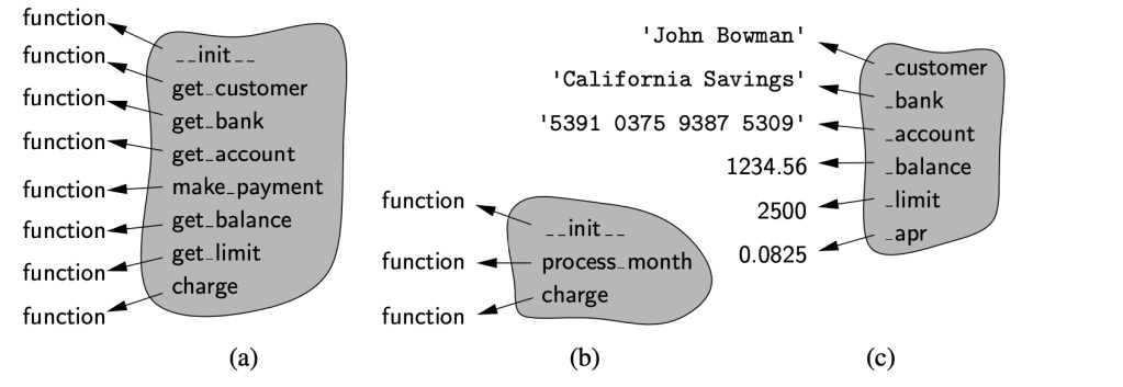
Three such namespaces: a class namespace containing methods of the CreditCard class, another class namespace with meth- ods of the PredatoryCreditCard class, and finally a single instance namespace for a sample instance of the PredatoryCreditCard class. We note that there are two different definitions of a function named charge, one in the CreditCard class, and then the overriding method in the PredatoryCreditCard class. In similar fashion, there are two distinct init implementations. However, process month is a name that is only defined within the scope of the PredatoryCreditCard class. The instance namespace includes all data members for the instance (including the apr member that is established by the PredatoryCreditCard constructor).
Shallow and Deep copying:
Take example of list warmtones:
red = 123
green = 222
brown =111
warmtones = [red,green,brown]
palette = list(warmtones)
In this case, we explicitly call the list constructor, sending the first list as a param- eter. This causes a new list to be created, as shown in Figure 2.10; however, it is what is known as a shallow copy. The new list is initialized so that its contents are precisely the same as the original sequence. However, Python’s lists are referential
We prefer that palette be what is known as a deep copy of warmtones. In a deep copy, the new copy references its own copies of those objects referenced by the original version.
All the SQL Server Agent Jobs details are logged into the MSDB Database tables .
These tables contains information for each SQL server Agent job like : JobID, sessionID, RunDate , Enabled Status, Owner, Job Steps, Last Run outcomes etc . Tables which are commonly used are :
We will be using the table ‘[HR].[Employees]’ from TSQL2012 database.
The error as described in the Title of the post :
"Msg 8120, Level 16, State 1, Line 1 Column 'HR.Employees.lastname' is invalid in the select list because it is not contained in either an aggregate function or the GROUP BY clause."
The error occured when I executed the following query :
select min(empid) as minimum,lastname from [HR].[Employees]
The reason for the error is : We are missing the group by clause at the end .When we are using an aggregate function along with other columns in the select clause we must use the group by clause .
select min(empid) as minimum,lastname from [HR].[Employees] group by lastname
If you are using more than one column in the select clause while using the aggregate function , then it is necessary to include all the columns in the group by clause except the column on which the aggregate function is applied. For instance : if you use execute the below query , it will throw the same error:
select min(empid) as minimum,lastname,firstname from [HR].[Employees] group by lastname
So , we must include the firstname column as well to successfully execute it as below :
select min(empid) as minimum,lastname,firstname from [HR].[Employees] group by lastname,firstname
This Error is very common when we insert or update data.
This error occurs when we try to insert data which is greater than the length of the column in which we are inserting the data.
For Instance : Lets see an example in our TSQL2012 database :
insert into [Production].Categories(categoryname,description) values ('No chocolate items','no chocolate')
It gave me an error :
Msg 8152, Level 16, State 4, Line 1
String or binary data would be truncated.
The statement has been terminated.
This happened because the Column Categoryname has the column type : nvarchar(15) , which means nvarchar can take upto 15 characters maximum. And the total length of characters tried to insert: ‘No chocolate items’ is of length 18 .
To solve this problem ,we can increase the length of column size to 18 . Or , we can reduce the characters accordingly to fit the size of 15 .
We will be working on the script attached during our posts . You can copy and paste the script in Microsoft SQL 2012 as we will be working on the tables , views , stored procedures , functions and other objects in the script.
Copy , paste and execute the whole script in a new MS SQL 2012 management Studio on the New Query tab to create the TSQL2012 database.
Attached is the script below in the TSQL2012.sql file .
The analyses of data from relational databases (LOB) applications is not an easy . The normalized relational schema used for an LOB application can consist of hundreds of tables. It is difficult to discover where the data you need for a report is located.
In addition, LOB applications do not track data over time(they perform many DML operations), though many analyses depend on historical data.
A Data warehouse is a centralized data database for an enterprise that contains merged, cleansed, and historical data. The DW data is more better for reporting purposes . The logical design of schema of DW is called Star schema and snowflake schema which consists of Dimension and fact Tables.
The data in DW comes from LOB / relational database . The data which comes in DW is more cleansed ,transformed . OF course , while coming into DW , the data must have gone through some changes so we can get the refreshed data in DW . One way to refresh or let the new data come into DW is through the night job schedule . The report for newly or refreshed data can then be read .
The physical design for the DW is simpler than the relational database design as it contains less tables joins .
————————————————————————————————————————————-
CHAPTER 1 : Introduction to Star and Snowflake Schemas
First learning why Reporting is a Problem with a Normalized Schema :
Lets take AdventureWorks2012 sample database . Now The report should include the sales amount for Internet sales in different countries over multiple years. This will end up with almost 10 tables. The AdventureWorks2012 database schema is very normalized; it’s intended as an example schema to support LOB applications.
The goal of normalization is to have a complete and non-redundant schema.
Every piece of information must be stored exactly once. This way, you can enforce data integrity.
So, a query that joins 10 to 12 tables, as would be required in reporting sales by countries
and years, would not be very fast and can cause performance issues as it reads huge amounts of data sales over multiple years and thus would interfere with the regular transactional work of insertion and updation of the data.
Another problem is in many cases, LOB databases are purged otypically after each new fiscal year starts. Even if you have all of the historical data for the sales transactions, you might have a problem showing the historical data correctly. For example, you might have only the latest customer address, which might prevent you from calculating historical sales by country correctly .
The AdventureWorks2012 sample database stores all data in a single database. However, in an enterprise, you might have multiple LOB applications, each of which might store data in its own database. You might also have part of the sales data in one database and part in another.
And you could have customer data in both databases, without a common identification. In such cases, you face the problems of how to merge all this data and how to identify which customer from one database is actually the same as a customer from another database.
Finally, data quality can be low. The old rule, “garbage in garbage out,” applies to analyses as well. Parts of the data could be missing; other parts could be wrong. Even with good data, you could still have different representations of the same data in different databases. For example, gender in one database could be represented with the letters F and M, and in another database with the numbers 1 and 2. So we can put a proper standard in our data warehouse to this problem.
Star Schema
In Figure below, you can easily identify how the Star schema as it resembles
a star. There is a single central table, called a fact table, surrounded by multiple tables called dimensions. One Star schema covers a particular business area. In this case, the schemacovers Internet sales. An enterprise data warehouse covers multiple business areas and consists of multiple Star and Snowflake schemas.
The fact table is connected to all the dimensions with foreign keys. Usually, all foreign keys taken together uniquely identify each row in the fact table, and thus they all together form a unique key, so you can use all the foreign keys as a composite primary key of the fact table. The fact table is on the “many” side of its relationships with the dimensions. If you were to form a proposition from a row in a fact table, you might express it with a sentence such as, “Customer CC purchased product BB on date DD in quantity QQ for amount SS.” .
As we know, a data warehouse consists of multiple Star schemas. From a business perspective, these Star schemas are connected. For example, you have the same customers in sales as in accounting. You deal with many of the same products in sales, inventory, and production. Of course, your business is performed at the same time over all the different business areas. To represent the business correctly, you must be able to connect the multiple Star schemas in your data warehouse. The connection is simple – you use the same dimensions for each Star schema. In fact, the dimensions should be shared among multiple Star schemas. Dimensions have foreign key relationships with multiple fact tables. Dimensions which have connections to multiple fact tables are called shared or conformed dimensions.
Snowflake Schema
You can imagine multiple dimensions designed in a similar normalized way, with a central fact table connected by foreign keys to dimension tables, which are connected with foreign keys to lookup tables, which are connected with foreign keys to their second-level lookup tables.
In this configuration, a star starts to resemble a snowflake. Therefore, a Star schema with normalized dimensions is called a Snowflake schema.
In most long-term projects, you should design Star schemas. Because the Star schema is
simpler than a Snowflake schema, it is also easier to maintain. Queries on a Star schema are simpler and faster than queries on a Snowflake schema, because they involve fewer joins.
Hybrid Schema
In some cases, you can also employ a hybrid approach, using a Snowflake schema only for the first level of a dimension lookup table. In this type of approach, there are no additional levels of lookup tables; the first-level lookup table is denormalized. Figure 1-6 shows such a partially denormalized schema.
Quick Question :
How do we connect multiple star schemas ?
Answer :
Through shared dimensions .
Granularity Level
The number of dimensions connected with a fact table defines the granularity level.
Auditing and Lineage
A data warehouse may also contain auditing tables. For every update, you should audit who and when the update was done and by whom and how many rows were affected to each dimension and fact table in your DW. If you also audit how much time was needed for each load, you can calculate the performance and take action if it slows down. You store this information in an auditing table .
You might also need to know where each row in a dimension and/or fact table came from and when it was added. In such cases, you must add appropriate columns to the dimension and fact tables. Such fine detailed auditing information is also called lineage.
Dimensions give context to measures. Typical analysis includes pivot tables and pivot graphs. These pivot on one or more dimension columns used for analysis—these columns are called attributes in DW and OLAP terminology.
Columns with unique values identify rows. These columns are keys. In a data warehouse, you need keys just like you need them in an LOB database. Keys uniquely identify entities. Therefore, keys are the second type of columns in a dimension.
Pivoting makes no sense if an attribute’s values are continuous, or if an attribute has too
many distinct values. Imagine how a pivot table would look if it had 1,000 columns, or how a pivot graph would look with 1,000 bars. For pivoting, discrete attributes with a small number of distinct values is most appropriate. A bar chart with more than 10 bars becomes difficult to comprehend. Continuous columns or columns with unique values, such as keys, are not appropriate for analyses.
If you have a continuous column and you would like to use it in analyses as a pivotingattribute, you should discretize it. Discretizing means grouping or binning values to a few discrete groups. If you are using OLAP cubes, SSAS can help you. SSAS can discretize continuous attributes. However, automatic discretization is usually worse than discretization from a business perspective. Age and income are typical attributes that should be discretized from a business perspective. One year makes a big difference when you are 15 years old, and much less when you are 55 years old. When you discretize age, you should use narrower ranges for younger people and wider ranges for older people(these are used for Graph type pivoting).
A customer typically has an address, a phone number, and an email address. You do notanalyze data on these columns. You do not need them for pivoting. However, you often need information such as the customer’s address on a report. If that data is not present in a DW, you will need to get it from an LOB database, probably with a distributed query. It is much simpler to store this data in your data warehouse. In addition, queries that use this data perform better, because the queries do not have to include data from LOB databases. Columns used in reports as labels only, not for pivoting, are called member properties.
In addition to the types of dimension columns already defined for identifying, naming,
pivoting, and labeling on a report, you can have columns for lineage information,
A dimension may contain the following types of columns:
■■ Keys Used to identify entities
■■ Name columns Used for human names of entities
■■ Attributes Used for pivoting in analyses
■■ Member properties Used for labels in a report
■■ Lineage columns Used for auditing, and never exposed to end users
Hierarchies
Figure 1-9 shows the DimCustomer dimension of the AdventureWorksDW2012 sample database.
In the figure, the following columns are attributes (columns used for pivoting):
■■ BirthDate (after calculating age and discretizing the age)
■■ MaritalStatus
■■ Gender
■■ YearlyIncome (after discretizing)
■■ TotalChildren
■■ NumberChildrenAtHome
■■ EnglishEducation (other education columns are for translations)
■■ EnglishOccupation (other occupation columns are for translations)
■■ HouseOwnerFlag
■■ NumberCarsOwned
■■ CommuteDistance
All these attributes are unrelated. Pivoting on MaritalStatus, for example, is unrelated to
pivoting on YearlyIncome. None of these columns have any functional dependency between them, and there is no natural drill-down path through these attributes. Now look at the Dim- Date columns, as shown in Figure 1-10.
Some attributes of the DimDate edimension include the following (not in the order shown in the figure):
■■ FullDateAlternateKey (denotes a date in date format)
■■ EnglishMonthName
■■ CalendarQuarter
■■ CalendarSemester
■■ CalendarYear
You will immediately notice that these attributes are connected. There is a functional dependency among them, so they break third normal form. They form a hierarchy. Hierarchies are particularly useful for pivoting and OLAP analyses—they provide a natural drill-down path. You perform divide-and-conquer analyses through hierarchies.
Hierarchies have levels. When drilling down, you move from a parent level to a child level. For example, a calendar drill-down path in the DimDate dimension goes through the following levels: CalendarYear ➝ CalendarSemester ➝ CalendarQuarter ➝ EnglishMonthName ➝ FullDateAlternateKey
At each level, you have members. For example, the members of the month level are, ofcourse, January, February, March, April, May, June, July, August, September, October, November, and December. In DW and OLAP jargon, rows on the leaf level—the actual dimension rows—are called members. This is why dimension columns used in reports for labels are called member properties.
In a Snowflake schema, lookup tables show you levels of hierarchies. In a Star schema, you need to extract natural hierarchies from the names and content of columns. Nevertheless, because drilling down through natural hierarchies is so useful and welcomed by end users, you should use them as much as possible.
Slowly Changing Dimensions
There is one common problem with dimensions in a data warehouse: the data in the dimension changes over time. This is usually not a problem in an OLTP application; when a piece of data changes, you just update it. However, in a DW, you have to maintain history. The question that arises is how to maintain it. Do you want to update only the changed data, as in an OLTP application, and pretend that the value was always the last value, or do you want to maintain both the first and intermediate values? This problem is known in DW jargon as the Slowly Changing Dimension (SCD) problem.
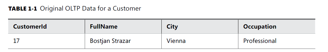
The problem is best explained in an example. Table 1-1 shows original source OLTP data
for a customer.
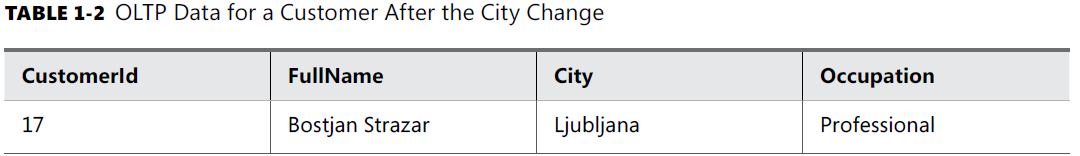
The customer lives in Vienna, Austria, and is a professional. Now imagine that the customer moves to Ljubljana, Slovenia. In an OLTP database, you would just update the City column, resulting in the values shown in Table 1-2.
If you create a report, all the historical sales for this customer are now attributed to the
city of Ljubljana, and (on a higher level) to Slovenia. The fact that this customer contributed to sales in Vienna and in Austria in the past would have disappeared.
In a DW, you can have the same data as in an OLTP database. You could use the same key,
such as the business key, for your Customer dimension. You could update the City column when you get a change notification from the OLTP system, and thus overwrite the history.
Type 1 SCD : Type 1 means overwriting the history for an attribute and for all higher levels of hierarchies to which that attribute belongs.
The problem here would rise that you want to store the historical data . What if we want transactions of the same customer when he did in Vienna ? The solution to this problem would be to add a surrogate key (DW key ).
Type 2 SCD : When you implement Type 2 SCD, for the sake of simpler querying, you typically also add a flag to denote which row is current for a dimension member. Alternatively, you could add two columns showing the interval of validity of a value.
You could have a mixture of Type 1 and Type 2 changes in a single dimension. For example, in Table 1-3, you might want to maintain the history for the City column but overwrite the history for the Occupation column. That raises yet another issue. When you want to update the Occupation column, you may find that there are two (and maybe more) rows for the same customer. The question is, do you want to update the last row only, or all the rows? Table 1-4 shows a version that updates the last (current) row only, whereas Table 1-5 shows all of the rows being updated.
Fact Table Column Types
Fact tables are collections of measurements associated with a specific business process. You store measurements in columns. Logically, this type of column is called a measure. Measures are the essence of a fact table. They are usually numeric and can be aggregated. They store values that are of interest to the business, such as sales amount, order quantity, and discount amount.
All foreign keys together usually uniquely identify each row and can be used as a composite primary key.
For example, suppose you start building a sales fact table from an order details table in a source system, and then add foreign keys that pertain to the order as a whole from the Order Header table in the source system. Tables 1-7, 1-8, and 1-9 illustrate an example of such a design process.
Table 1-7 shows a simplified example of an Orders Header source table. The OrderId
column is the primary key for this table. The CustomerId column is a foreign key from the Customers table. The OrderDate column is not a foreign key in the source table; however, it becomes a foreign key in the DW fact table, for the relationship with the explicit date dimension. Note, however, that foreign keys in a fact table can—and usually are—replaced with DW surrogate keys of DW dimensions.
Table 1-8 shows the source Order Details table. The primary key of this table is a composite one and consists of the OrderId and LineItemId columns. In addition, the Source Order Details table has the ProductId foreign key column. The Quantity column is the measure .
Table 1-9 shows the Sales Fact table created from the Orders Header and Order Details
source tables. The Order Details table was the primary source for this fact table. The OrderId, LineItemId, and Quantity columns are simply transferred from the source Order Details table.
The ProductId column from the source Order Details table is replaced with a surrogate DW ProductKey column. The CustomerId and OrderDate columns take the source Orders Header table; these columns pertain to orders, not order details. However, in the fact table, they are replaced with the surrogate DW keys CustomerKey and OrderDateKey.
You do not need the OrderId and LineItemId columns in this sales fact table. For analyses, you could create a composite primary key from the CustomerKey, OrderDateKey, and Product- Key columns.
Additivity of Measures
Additivity of measures is not exactly a data warehouse design problem. However, you should consider which aggregate functions you will use in reports for which measures, and which aggregate functions you will use when aggregating over which dimension.
The simplest types of measures are those that can be aggregated with the SUM aggregate
function across all dimensions, such as amounts or quantities. For example, if sales for product A were $200.00 and sales for product B were $150.00, then the total of the sales was $350.00. If yesterday’s sales were $100.00 and sales for the day before yesterday were $130.00, then the total sales amounted to $230.00. Measures that can be summarized across all dimensions are called additive measures.
Some measures are not additive over any dimension. Examples include prices and percentages, such as a discount percentage. Typically, you use the AVERAGE aggregate function for such measures, or you do not aggregate them at all. Such measures are called non-additive measures.
For some measures, you can use SUM aggregate functions over all dimensions but time.
Some examples include levels and balances. Such measures are called semi-additive measures. For example, if customer A has $2,000.00 in a bank account, and customer B has $3,000.00, together they have $5,000.00. However, if customer A had $5,000.00 in an account yesterday but has only $2,000.00 today, then customer A obviously does not have $7,000.00 altogether. You should take care how you aggregate such measures in a report. For time measures, you can calculate average value or use the last value as the aggregate.
Quick Question :
■■ You are designing an accounting system. Your measures are debit, credit, and
balance. What is the additivity of each measure?
Answer: Debit and credit are additive measure while balance is semi additive measure.
Summary :
■■ Fact tables include measures, foreign keys, and possibly an additional primary key and lineage columns.
■■ Measures can be additive(fixed total sum of sales ) , non-additive(price changes or percentage changes ), or semi-additive(credit and debit in account) 32