Creating a Data Warehouse Database

A DW is a transformed  (LOB) data. You load data to your DW  on a schedule mostly in an overnight job. The DW data is not online, real-time data. You do not need to back up the transaction log for your data warehouse, as you would in an LOB database. Therefore, the recovery model for your data warehouse should be Simple.

■■ In the Full recovery model, all transactions are fully logged, with all associated data. You have to regularly back up the log. You can recover data to any arbitrary point in time. Point-in-time recovery is particularly useful when human errors occur.

■■ The Bulk Logged recovery model is an adjunct of the Full recovery model that permits
high-performance bulk copy operations. Bulk operations, such as index creation or
bulk loading of text or XML data, can be minimally logged. For such operations, SQL
Server can log only the Transact-SQL command, without all the associated data. You
still need to back up the transaction log regularly.

■■ In the Simple recovery model, SQL Server automatically reclaims log space for committed transactions. SQL Server keeps log space requirements small, essentially eliminating the need to manage the transaction log space.

In your data warehouse, large fact tables typically occupy most of the space. You can
optimize querying and managing large fact tables through partitioning. Table partitioning has management advantages and provides performance benefits. Queries often touch only subsets of partitions, and SQL Server can efficiently eliminate other partitions early in the query execution process.

A database can have multiple data files, grouped in multiple filegroups. There is no single best practice as to how many filegroups you should create for your data warehouse. However, for most DW scenarios, having one filegroup for each partition is the most appropriate. For the number of files in a filegroup, you should consider your disk storage. Generally, you should create one file per physical disk.

Loading data from source systems is often quite complex. To mitigate the complexity,
you can implement staging tables in your DW. You can even implement staging tables and other objects in a separate database. You use staging tables to temporarily store source data before cleansing it or merging it with data from other sources. In addition, staging tables also serve as an intermediate layer between DW and source tables. If something changes in the source—for example if a source database is upgraded—you have to change only the query that reads source data and loads it to staging tables. After that, your regular ETL process should work just as it did before the change in the source system. The part of a DW containing staging tables is called the data staging area (DSA).

Implementing Dimensions

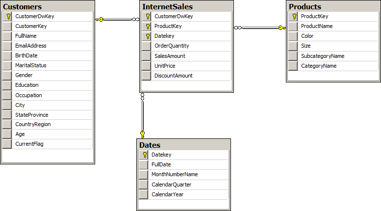
Implementing a dimension involves creating a table that contains all the needed columns. In addition to business keys, you should add a surrogate key to all dimensions that need Type 2 Slowly Changing Dimension (SCD) management. You should also add a column that flags the current row or two date columns that mark the validity period of a row when you implement Type 2 SCD management for a dimension.

You can use simple sequential integers for surrogate keys. SQL Server can autonumber them for you. You can use the IDENTITY property to generate sequential numbers.

A sequence is a user-defined, table-independent (and therefore schema-bound) object.
SQL Server uses sequences to generate a sequence of numeric values according to your specification. You can generate sequences in ascending or descending order, using a defined interval.of possible values. You can even generate sequences that cycle (repeat).

As mentioned, sequences are independent objects, not associated with tables. You control the relationship between sequences and tables in your ETL application. With sequences, you can coordinate the key values across multiple tables.
You should use sequences instead of identity columns in the following scenarios:
■■ When you need to determine the next number before making an insert into a table.

■■ When you want to share a single series of numbers between multiple tables.

■■ When you need to restart the number series when a specified number is reached (that is, when you need to cycle the sequence).

Implementing Fact Tables

After you implement dimensions, you need to implement fact tables in your data warehouse. You should always implement fact tables after you implement your dimensions. A fact table is on the “many” side of a relationship with a dimension, so the parent side must exist if you want to create a foreign key constraint.

You should partition a large fact table for easier maintenance and better performance.

Columns in a fact table include foreign keys and measures. Dimensions in your database
define the foreign keys. All foreign keys together usually uniquely identify each row of a fact table.

In production, you can remove foreign key constraints to achieve better load performance.
If the foreign key constraints are present, SQL Server has to check them during the load. However, we recommend that you retain the foreign key constraints during the development and testing phases. It is easier to create database diagrams if you have foreign keys defined. In addition, during the tests, you will get errors if constraints are violated. Errors inform you that there is something wrong with your data; when a foreign key violation occurs, it’s most likely that the parent row from a dimension is missing for one or more rows in a fact table. These types of errors give you information about the quality of the data you are dealing with.
If you decide to remove foreign keys in production, you should create your ETL process
so that it’s resilient when foreign key errors occur. In your ETL process, you should add a row to a dimension when an unknown key appears in a fact table. A row in a dimension added during fact table load is called an inferred member. Except for the key values, all other column Key values for an inferred member row in a dimension are unknown at fact table load time, and you should set them to NULL. This means that dimension columns (except keys) should allow NULLs.

Columnstore Indexes and Batch Processing

A columnstore index is just another nonclustered index on a table. Query Optimizer considers using it during the query optimization phase just as it does any other index .

A columnstore index is often compressed even further than any data compression type
can compress the row storage—including page and Unicode compression. When a query
references a single column that is a part of a columnstore index, then SQL Server fetches only that column from disk; it doesn’t fetch entire rows as with row storage. This also reduces disk IO and memory cache consumption. Columnstore indexes use their own compression algorithm; you cannot use row or page compression on a columnstore index.

On the other hand, SQL Server has to return rows. Therefore, rows must be reconstructed when you execute a query. This row reconstruction takes some time and uses some CPU and memory resources. Very selective queries that touch only a few rows might not benefit from columnstore indexes. Columnstore indexes accelerate data warehouse queries but are not suitable for OLTP workloads.

The columnstore index is divided into units called segments. Segments are stored as large objects, and consist of multiple pages. A segment is the unit of transfer from disk to memory.
Each segment has metadata that stores the minimum and maximum value of each column for that segment. This enables early segment elimination in the storage engine. SQL Server loads only those segments requested by a query into memory.

SQL Server 2012 includes another important improvement for query processing. In batch mode processing, SQL Server processes data in batches rather than processing one row at a time. In SQL Server 2012, a batch represents roughly 1000 rows of data. Each column within a batch is stored as a vector in a separate memory area, meaning that batch mode processing is vector-based. Batch mode processing interrupts a processor with metadata only once per batch rather than once per row, as in row mode processing, which lowers the CPU burden substantially.

Loading and Auditing Loads

Loading large fact tables can be a problem. You have only a limited time window in which to do the load, so you need to optimize the load operation. In addition, you might be required to track the loads.

Using Partitions

Loading even very large fact tables is not a problem if you can perform incremental loads. However, this means that data in the source should never be updated or deleted; data should be inserted only. This is rarely the case with LOB applications. In addition, even if you have the possibility of performing an incremental load, you should have a parameterized ETL procedure in place so you can reload portions of data loaded already in earlier loads. There is always a possibility that something might go wrong in the source system, which means that you will have to reload historical data. This reloading will require you to delete part of the data from your data warehouse.

Deleting large portions of fact tables might consume too much time, unless you perform a minimally logged deletion. A minimally logged deletion operation can be done by using the TRUNCATE TABLE command; however, this command deletes all the data from a table—and deleting all the data is usually not acceptable. More commonly, you need to delete only portions of the data.

Inserting huge amounts of data could consume too much time as well. You can do a minimally logged insert, but as you already know, minimally logged inserts have some limitations. Among other limitations, a table must either be empty, have no indexes, or use a clustered index only on an ever-increasing (or ever-decreasing) key, so that all inserts occur on one end of the index. However, you would probably like to have some indexes on your fact table—at least a columnstore index. With a columnstore index, the situation is even worse—the table becomes read only.

You can resolve all of these problems by partitioning a table. You can even achieve better
query performance by using a partitioned table, because you can create partitions in different filegroups on different drives, thus parallelizing reads. You can also perform maintenance procedures on a subset of filegroups, and thus on a subset of partitions only. That way, you can also speed up regular maintenance tasks. Altogether, partitions have many benefits.

Although you can partition a table on any attribute, partitioning over dates is most common in data warehousing scenarios. You can use any time interval for a partition. Depending on your needs, the interval could be a day, a month, a year, or any other interval. You can have as many as 15,000 partitions per table in SQL Server 2012.

In addition to partitioning tables, you can also partition indexes. Partitioned table and
index concepts include the following:

■■ Partition function : This is an object that maps rows to partitions by using values
from specific columns. The columns used for the function are called partitioning columns. A partition function performs logical mapping.

■■ Partition scheme : A partition scheme maps partitions to filegroups. A partition
scheme performs physical mapping.

■■ Aligned index : This is an index built on the same partition scheme as its base table.
If all indexes are aligned with their base table, switching a partition is a metadata operation only, so it is very fast. Columnstore indexes have to be aligned with their base
tables. Nonaligned indexes are, of course, indexes that are partitioned differently than
their base tables.

■■ Partition elimination : This is a Query Optimizer process in which SQL Server accesses only those partitions needed to satisfy query filters.

■■ Partition switching  : This is a process that switches a block of data from one table or
partition to another table or partition. You switch the data by using the ALTER TABLE T-SQL command. You can perform the following types of switches:
■ Reassign all data from a nonpartitioned table to an empty existing partition of a partitioned table.
■ Switch a partition of one partitioned table to a partition of another partitioned table.
■ Reassign all data from a partition of a partitioned table to an existing empty nonpartitioned table.

Any time you create a large partitioned table you should create two auxiliary nonindexed empty tables with the same structure, including constraints and data compression options.

For minimally logged deletions of large portions of data, you can switch a partition from
the fact table to the empty table version without the check constraint. Then you can truncate that table. The TRUNCATE TABLE statement is minimally logged. Your first auxiliary table is prepared to accept the next partition from your fact table for the next minimally logged deletion.

For minimally logged inserts, you can bulk insert new data to the second auxiliary table,
the one that has the check constraint. In this case, the INSERT operation can be minimally
logged because the table is empty. Then you create a columnstore index on this auxiliary
table, using the same structure as the columnstore index on your fact table. Now you can
switch data from this auxiliary table to a partition of your fact table. Finally, you drop the columnstore index on the auxiliary table, and change the check constraint to guarantee that all of the data for the next load can be switched to the next empty partition of your fact table. Your second auxiliary table is prepared for new bulk loads again.

• 9. Data Warehouse - 1