An object is an Entity, for example: car, house , person, time etc. Object can be tangible or intangible.
Lets consider a car (tangible) which is our object . An object has an attribute, behaviour and has a unique Id.
Car has attribute (color, model) , behaviour ( accelerate, brake the car, change gear) and has a unique registration number.
Now , lets take an intangible object example: Time. A time can have attributes like: Year, month, day. A time can have its behaviour set, like set the Year, set the Month, set the day and it can have a unique identifier : Date of birth, date of joining the college, date of creation.
- Information hiding:
Some characteristics of object are:
Information is stored within an object.
It is hidden from outside world.
It can only be manipulated by the object itself.
Example: An object called Alex who is a person and he is our object model, the outside world or any other person cannot know his name by seeing him or interacting with him. We cannot also know his exact age until he lets us know. We can get his name and age only when he wants us to let us know. So, we cannot access his name and age directly but we can ask him to tell his name.
Another example is contact numbers stored on a mobile phone. A mobile phone is an object. It is hiding phone numbers inside it. If i want to get a number starting from letter ‘S’ then i have to ask or access the phone to get me the list of numbers starting from ‘S’.
So information hiding simplifies the process. An object Alex enquires from object phone to tell him the numbers starting from ‘S’. So in short, Alex’s information like age or name is hidden until he tells you or he gives access to his details and you cannot access the phone numbers until you get access to the phone itself and perform the operations.
2. Encapsulation:
State and behaviour of an object are tightly coupled. You can perceive an object whose name is Alex and age is 36. You do not know how he has stored that information in his brain, when you ask him , he performs that operation and then lets you know his name and age. You do not know in which part of the brain he has that information and how he got it.
A phone has stored a phone number in digital format and knows how to convert in human readable format. A user does know how data is stored and how it is converted to human readable format.
3. Object has an interface:
An object encapsulates data and behaviour. So how objects interact with each other ? Each object provides an interface (operations).
So lets say , an object whose name is Alex. You ask Alex in english , what is your name ? So he will tell you his name. If you ask him any other thing like where are you going or what is your plan , you will never get his name. So in simple terms the only interface which Alex has allowed to get exposed to you or outer world is by asking what is your name. Any other way you try to get his name , you will not get it.
Another example can be: an object car , whose interface can be : Steer wheels, change gear, accelerate, apply brakes.
If you want to speed up the car you have to accelerate. If you want to change the direction of the car you will use its interface steer wheels, if you have to stop the car you have to apply the brakes interface, you cannot stop the car if you try to use any other interface!
Abstraction:
Abstraction is a way to cope with complexity and reduce the complexity .
Principle of abstraction: Capture those details about an object that are relevant to that perspective.
For example: Alex is a student of PhD in a school and teaches some undergrad student courses. He might be having attributes like studentId, badge no, age, year,CGPA, Employee Id, designation, salary.
So it seems he is a student as well as a teacher in the school. There can be other more perspectives to the object Alex, like his sports playing perspectice like his score, his match date, his jersey no. There can be his medical perspectives like his height, age, blood group, his vaccination dates etc. These are different perspectives related to Alex. To make things simple in OOP, we only relate the object to its perspective and this way we make things simple.
Lets take the example we highlighted in bold , where Alex is a PhD student as well as a teacher. There are two perspectives one as a student (studentId, badge no, age, year, CGPA) and one as a teacher(EmployeeId, designation, salary).Similarly , Alex’s behaviour as a student can be: study, play sports, give exams.
Alex’s behaviour as a teacher can be deliver lecture, prepare exam, teach and take exam.
Lets take another example : A car with a driver’s perspective and engineer’s perspective.
Driver’s perspective: A car has 4 doors, white color, a steering wheel, good seats.
Engineer’s perspective: Structure of car, engine, number of rods, wheel type etc .
So each perspective is separate and making them separate will reduce complexity.
Classes:
In OOP Model: Some of the Objects exhibit identical characteristics ( information structure and behaviour).
We say they belong to the same class.
For example: There are 15 students in a class room. They exhibit almost same behaviour, they take notes, sit on a chair and give the exam. So we can instantiate each student as an object with identical characteristics.
Take another example of a wooden stamp which has a government seal. When you stamp it , it creates a different object but the characteristic is same, the government seal.
So, take an example: A student class , there are three students , Alex who studies maths, Katherine who studies chemistry and Jack studies Physics. We created three objects here as an instance of student class.
Inheritance:
A child inherits characteristics of his parents.
Besides that a child may also have its own unique characteristics.
If class B inherits from class A, then class B will have all characteristics (attributes and behaviour) of class A . A parent class is called Base class and child class is called derived class.
Consider a Parent class Person having its child classes student, teacher and doctor.
A parent class shape having child classes circle, triangle and line.
A person parent class has (name,age, eat( ), walk( ) ) has a derived class student (class, year, study( ), give exam( ) ) and a class teacher (employeeId, designation, teach( ), take exam( ) ).
- Generalization in Inheritance:
The derived class inherit general characteristics.
A teacher and a student both eat and walk. So we can put these characteristics in a base class called person.
Person(name,age, gender, walk( ), eat( ) ) .
Student (program,year, give exam( ), study( ) ) and Teacher( designation, employee Id, take exam( ), teach( ) ).
Student is a person. Teacher is a person.
2. Subtyping( Extension) :
Sub-typing means that derived class is behaviourally compatible with base class. Behaviourally compatible means that base class can be replaced by derived class.
3. Speciaization (Restriction):
Specialization means that derived class is behaviourally incompatible with base class.And it means that base class cannot always be replaced by derived class.
Suppose a base class called Person has a derived class Adult. Person <– Adult , now if we add a restriction in adult class that age < 18 then it cannot be an adult , so Person class then cannot be replaced by Adult class.
Another example is base class called Integer Set (add(element) ) which has derived class called Natural Set( add(element) ).
Integer Set (add element( ) ) <– Natural Set (add element( ) ).
Consider an integer Set class which includes negative, zero and positive numbers. Now lets look at Natural set ,which can only include 0,1,2,3 and so on.. It cannot include negative numbers. So a Natural Set class is a specialized class of Integer Set class.
4. Overriding:
A derived class may override a default behaviour from its parent class but may exhibit totally new behaviour or new implementation. This is called overriding.
The reasons for overriding can be:
Provide a new behaviour specific to the derived class
Restricting default behaviour.
Extend the default behaviour.
Improve performance.
For example : In Integer Set class we use add(element) to add two variables but in Natural Set we can use to add 5 elements.
Overriding concept is under inheritance in OO modeling not outside it.
Abstract Classes
An abstract class implements abstract concept.
Main purpose is to be inherited by other classes.
Cannot be instantiated.
Promotes re use.
In the person and student,teacher , doctor classes example, person class can be an abstract class. Firstly the abstract class are mostly at top of the hierarchy so it can be inherited. A person class can be an abstract class because in real life for example : we say he is a doctor , he is a student , she is a teacher, not he is a person, she is a person.
Take another example of a shape class which has a derived class called circle, line, triangle. We do not say it is a shape when we see a circle or a triangle in real life. We say it is a circle or a triangle.
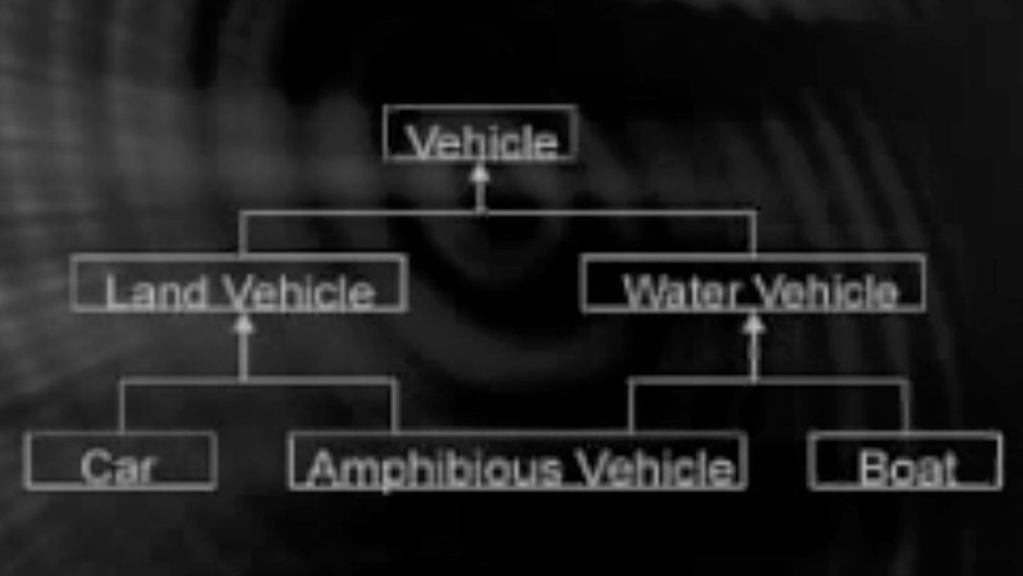
Another example: class vehicle(color,model,year, accelerate( ), brake( ) ) , car(color, model, year, accelerate( ), brake( )), truck(color, model, year, accelerate( ), brake( )).
That is why we keep abstract class at the top because it exhibits general , common concept like : shape, person, vehicle.
Rather than the classes from which we can create objects from are called concrete classes. Like teacher , doctor, student from Person class . Car, truck , cycle from vehicle class. So we instantiate object from a concrete class .
Multiple Inheritance:
A class inherited from multiple classes is said to have multiple inheritance. For example : If i have to create a mermaid i have to inherit properties of a human and a fish. So in OO model a mermaid class will be made from human class and a fish class.
Association:
Alex drives a car. It can have 1….* association. Alex can drive his car or any other car.
Association can be two way, if Alex is friend of Katty then Katty is also friend of Alex.And this is 1..1 is a two way association.
There can be ternary association as well. For example: Student, course and teacher. Student * .. 1 teacher, Course *…1 teacher. One teacher can teach multiple courses to multiple students.
Composition:
An object may be composed of smaller objects.
The relationship between part objects and whole object is known as composition.
Composition is represented by a filled diamond towards the composed object. It is a strong relationship.
For example: Alex is composed of parts called: 2 legs, 2 arms, 1 head and 1 body.
Aggregation:
An object may contain collection(aggregate) of other objects.
The relationship between container and the contained object is called aggregation. And it is represented by an unfilled diamond towards the container object.
An room contains bed, a cupboard and chairs. But it is not formed or made with these objects. It contains it.
A garden contains many plants. It contains them.
Aggregation is a weaker relationship as it contains the items but not formed from it. Why we say it a weak relationship is because if we remove the room , we can still use the chair and the cupboard. Or we remove these items from the room we can still use the room.
Polymorphism
Polymorphism refers to existence of different forms of same entity.
Diamond and coal are different forms of Carbon.
It is a powerful tool to develop flexible and resusable system.
For example: you have open an editor and there is a print option , whatever file is open either a pdf file, png file or word file, it will print depending on the object.
We can add or create new objects depending on the requirement.
Lets take another example: We have shape class , and its derived class triangle, circle , line . Now we want to add a new derived class square. We can use the same draw( ) method . System will use the draw( ) depending on the object.
Lets work with examples now with Python:
Creating Object:
Instantiation:
The process of creating a new object of a class is called instantiation.
Consider a class as a blueprint and the object instance as a physical object.
When you create an object instance it allocates a space for that object in the memory.
It then calls its constructor function which is a special function with __init__( ) as a syntax in python, it initializes an initial state for the newly created object. Think of a constructor that it sets an initial stage. If we do not initialize or set attributes in constructor then we have to manually write that attributes value every time.
For example:
# without constructorclass Robot: passrobot = Robot()robot.name="Optimus"robot.battery = 100# with constructorclass Robot:def__init__(self,name,battery=100): self.name= name self.battery = batteryrobot = Robot("optimus")
Many of Python’s built-in classes support what is known as a literal form for designating new instances. For example, the command temperature = 98.6 results in the creation of a new instance of the float class; the term 98.6 in that expression is a literal form.
From a programmer’s perspective, yet another way to indirectly create a new instance of a class is to call a function that creates and returns such an instance. For example, Python has a built-in function named sorted that takes a sequence of comparable elements as a parameter and returns a new instance of the list class containing those elements in sorted order.
Functions:
When using a method of a class, it is important to understand its behavior. Some methods return information about the state of an object, but do not change that state. These are known as accessors. Other methods, such as the sort method of the list class, do change the state of an object. These methods are known as mutators or update methods.
Python’s Built-In Classes
Table provides a summary of commonly used, built-in classes in Python; we take particular note of which classes are mutable and which are immutable. A class is immutable if each object of that class has a fixed value upon instantiation that cannot subsequently be changed. For example, the float class is immutable. Once an instance has been created, its value cannot be changed (although an identifier referencing that object can be reassigned to a different value).
| Class | Description | Immutable? |
| bool | Boolean value | Immutable |
| int | integer (arbitrary magnitude) | Immutable |
| float | floating-point number | Immutable |
| list | mutable sequence of objects | Mutable |
| tuple | immutable sequence of objects | Immutable |
| str | character string | Immutable |
| set | unordered set of distinct objects | Mutable |
| frozenset | immutable form of set class | Immutable |
| dict | associative mapping (aka dictionary) | Mutable |