Author: ahmed7

Review Topics for SSAS – OLAP

SSAS works best with database schemas that are designed to support data analytics and reporting needs. You achieve such schemas by reducing the number of tables available for reporting, denormalizing data, and simplifying the database schema. The methodology you use to architect such schemas is called dimensional modeling.

After the dimensional schema is in place, you can build the Unified Dimensional Model
(UDM), also known as an SSAS cube, on top of it. The cube is a logical storage object that combines dimensions and measures to provide a multidimensional view of data .

The UDM consists of several components, as follows:

Data source Represents a connection to the database where the data is stored. SSAS uses the data source to retrieve data and load the UDM objects when you process them.

Data source view (DSV ) : It is just like views. Abstracts the underlying database schema. Although a DSV might seem redundant, it can be very useful by letting you augment the schema. For example, you can add calculated columns to a DSV when security policies prevent you from changing the database schema .

A data source view consists of a set of one or more logical tables with each table representing a saved SQL select statement. This feature has a number of advantages. It allows you to add or modify the underlying database design to fit your current needs without breaking the cubes. If the underlying database changes, modify the data source view to present the database as it was before the change. Additionally, if the data warehouse is not designed the way you would like it to be, you can modify the data source view to mimic your ideal data warehouse design.

Dimensional model :After you’ve created a DSV, the next step is to build the cube
dimensional model. The result of this process is the cube definition, consisting of measures and dimensions with attribute and/or multilevel hierarchies.

Named Queries : Each data source view table is a select statement. You can modify these select statements and join data to them from more than one SQL Server table. In our example, the Titles dimension includes both the DimTitles and DimPublishers tables in a snowflake pattern .

Named Calculation : As its name suggests, a named calculation is a column based on an expression.Named calculations allow you to modify a portion of the underlying SQL statement that is used by a data source view. A named calculation is similar to a named query, except that you add only a SQL expression to an existing statement, rather than using a whole SQL statement.

sql1 sql2

Dimensions

The Attributes :

KeyColumns : A collection of one or more columns uniquely identifying one row from
another in the dimension table (for example, 1, 2, or 3).

Name :The logical name of an attribute.

NameColumn: The values that are displayed in the client application when a particular
attribute is selected (for example, Red, Green, or Blue).

Type : The type of data the attribute represents (for example, day, month, or year) .

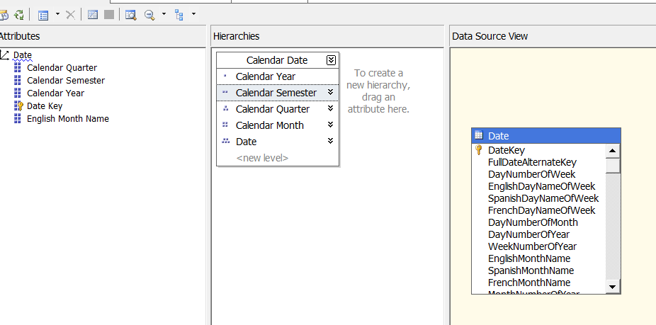
The Hierarchies Pane :

When you first create a dimension, each attribute is independent of each other, but user hierarchies allow you to group attributes into one or more parent-child relationships. Each relationship forms a new level of the hierarchy and provides reporting software with a way to browse data as a collection of levels-based attributes .

sql4

Cubes:

After the cube has been created, the cube needs to be configured and validated. Configuring a cube means modifying the cube to fit your needs, whereas validating a cube means verifying that the cube’s configuration is viable.

Cube Structure : Sets the properties for measures and measure groups
Dimension Usage: Maps connections between each dimension and measure group
Calculations :Adds additional MDX calculations to your cube
KPIs: Adds key performance indicator measures to your cube
Actions :Adds additional actions such as drill through and hyperlinks
Partitions :Divides measures and dimensions for fine-tuning aggregations to be stored
on the hard drive.
Aggregations :Finds which aggregations should be stored on the hard drive
Perspectives Defines SQL view–like structures for your cube.
Translations : Adds additional natural languages to the captions of your cube
Browser Browses the cube from the development environment .

Calculated members :

The Calculations tab enables you to create named MDX expressions, also known as calculated members . Typically these calculated members are used to create additional measures, but they can also be used to create additional dimensional attributes.

An example of an additional measure is acquiring the total price of an individual sale by multiplying the quantity by the price of the product. An additional dimensional member example is combining countries into groups such as combining Mexico, Canada, and the United States into one member called North America.

By default, all new calculated members are created on the Measures dimension. Calculated members in the Measures dimension go by a special name, known as calculated measures.

calcmeasure

Calculated Members vs. Derived Members

Calculated members use MDX expressions to create new members to the measures or other dimensions.
Derived members use SQL expressions to create new members on the measures or other dimensions. Derived members are created in SSAS by modifying the SQL code behind each table in a data source view. This can be somewhat confusing, so let’s review the difference between calculated members and derived members.

Listing 11-3. SQL Code for a Derived Measure
SELECT
FactSales.OrderNumber
, FactSales.OrderDateKey
, FactSales.TitleKey
, FactSales.StoreKey
, FactSales.SalesQuantity
— Adding derived measures
, DimTitles.TitlePrice as [CurrentStdPrice]
, (DimTitles.TitlePrice * FactSales.SalesQuantity) as DerivedTotalPrice
FROM FactSales
INNER JOIN DimTitles
ON FactSales.TitleKey = DimTitles.TitleKey

KPIs :A key performance indicator (KPI) is a way of grouping measures together into five basic categories. The five basic categories start at -1 and proceed to a +1 using an increment of ( -1, -0.50, 0, +0.50, and +1). The numbering system may seem odd to some, but it has to do with the science of statistics. Because of this, SSAS uses only these five categories, and they cannot be redefined.

The idea behind a KPI is for you to reduce the number of individual values in a tabular report to the essence of those values. This is convenient when you have a large report and what you really want to see is whether something has achieved a predefined target value, exceeded it, or did not make it to that value.
KPIs can be created in programming code such as SQL, C#, or MDX. In Listing 11-4 , you can see an example of an MDX statement that defines a range of values and categorizes each value within that range as either -1, 0, or 1. To keep things simple, we excluded the .05 and -05 categories and will work with just these three categories for now.

Listing 11-4. MDX Statement That Groups Values into Three KPI Categories
WITH MEMBER [MyKPI]
AS
case
when [SalesQuantity] < 25 or null then -1
when [SalesQuantity] > = 25 and [SalesQuantity] < = 50 then 0
when [SalesQuantity] > 50 then 1
end
SELECT
{ [Measures].[SalesQuantity], [Measures].[MyKPI] } on 0,
{ [DimTitles].[Title].members } on 1
From[CubeDWPubsSales]

kpi1

The number 493 is greater than 25 to 50; therefore, the status indicator is an upward-pointing arrow .

Often KPIs have the following five commonly used properties: 

Name: Indicates the name of the Key Performance Indicator. 

Actual/Value: Indicates the actual value of a measure pre-defined to align with organizational goals. 

Target/Goal: Indicates the target value (i.e. goal) of a measure pre-defined to align with organizational goals. 

Status: It is a numeric value and indicates the status of the KPI like performance is better than expected, performance is as expected, performance is not as expected, performance is much lower than expected, etc. 

Trend: It is a numeric value and indicates the KPIs trend like performance is constant over a period of time, performance is improving over a period of time, performance is degrading over a period of time, etc.

Apart from the above listed properties, most of the times, KPIs contain the following two optional properties:  Status Indicator: It is a graphical Indicator used to visually display the status of a KPI. Usually colors like red, yellow, and green are used or even other graphics like smiley or unhappy faces.  Trend Indicator: It is a graphical indicator used to visually display the trend of a KPI. Usually up arrow, right arrow, and down arrow are used.

Partitions :

The Partitions tab allows you to create and configure cube partitions. Partitions are a way of dividing a cube into one or more folders. These folders are usually placed on one or more hard drives and independently configured for increased performance.

Partition Storage Designs

In this dialog window you can choose how data is stored for a particular partition. Partition data falls into three categories of data: leaf level (individual values), aggregated total and subtotal values, and metadata that describes the partition.
Data storage designs also fall into three categories: MOLAP, HOLAP, and ROLAP (Figure 12-16). Storage locations, however, fall into two categories: an SSAS database folder or tables in a relational database.

rolap

There are primarily two types of data in SSAS: summary and detail data. Based on the approach used to store each of these two types of data, there are three standard storage modes supported by partitions: 

ROLAP: ROLAP stands for Real Time Online Analytical Processing. In this storage mode, summary data is stored in the relational data warehouse and detail data is stored in the relational database. This storage mode offers low latency, but it requires large storage space as well as slower processing and query response times. 

MOLAP: MOLAP stands for Multidimensional Online Analytical Processing. In this storage mode, both summary and detail data is stored on the OLAP server (multidimensional storage). This storage mode offers faster query response and processing times, but offers a high latency and requires average amount of storage space. This storage mode leads to duplication of data as the detail data is present in both the relational as well as the multidimensional storage. 

HOLAP: HOLAP stands for Hybrid Online Analytical Processing. This storage mode is a combination of ROLAP and MOLAP storage modes. In this storage mode, summary data is stored in OLAP server (Multidimensional storage) and detail data is stored in the relational data warehouse. This storage mode offers optimal storage space, query response time, latency and fast processing times.

Perspectives :

Perspectives are a named selection of cubes, dimensions, and measures. These are similar to a SQL view in that they allow you to filter what can and cannot be seen by the perspective. By default, whenever you create a cube, users can see every dimension and measure within that cube. If the cube has a lot of measures and dimensions, this can be confusing for your cube report builders. You could make several cubes in the same database, but perspectives allow you to select a subset of cubes, dimensions, and measures.

Translations:

Translations are very useful in achieving higher level of adoption of the BI/Analytics system (SSAS). This will eliminate the language barriers among users from different locations/languages and presents the same information in different languages making single version of truth available to users across different geographical locations.

Role Playing Dimensions:

A Role-Playing Dimension is a Dimension which is connected to the same Fact Table multiple times using different Foreign Keys. This helps the users to visualize the same cube data in different contexts/angles to get a better understanding and make better decisions.

Reference Dimensions :

Reference dimensions allow you to create a dimension that is indirectly linked to a fact table. To accomplish this, you must identify an intermediate dimension table. As an example, we use the DimCategories table, which is indirectly connected to the FactOrders table through the DimProducts table.

Interview Questions -1

1 – Query the list of CITY names starting with vowels (i.e., a, e, i, o, or u) from STATION. Your result cannot contain duplicates.

Answer : select city from station where city like ‘[aeiou]%’

2 – Query the names of all American cities in CITY with populations larger than 120000. The CountryCode for America is USA.

Answer : select name from city where countrycode =’USA’ and population > 120000

3 – Query a list of CITY names from STATION with even ID numbers only. You may print the results in any order, but must exclude duplicates .

Answer : select distinct city from station where id % 2=0 order by city

4 – Query the two cities in STATION with the shortest and longest CITY names, as well as their respective lengths (i.e.: number of characters in the name). If there is more than one smallest or largest city, choose the one that comes first when ordered alphabetically.

Input Format

The STATION table is described as follows:

Sample Output

ABC 3
PQRS 4

Answer : select top 1 city,LEN(city) from STATION order by len(city),city;
select top 1 city,LEN(city) from STATION order by len(city) desc

5 – Query the Name of any student in STUDENTS who scored higher than Marks. Order your output by the last three characters of each name. If two or more students both have names ending in the same last three characters (i.e.: Bobby, Robby, etc.), secondary sort them by ascending ID.

select name
from students
where marks>75 and name=’Stuart’
order by substring(name,len(name)-2, 3) , id asc;

Explanation of Substring : SELECT substring(‘W3Schools.com’,LEN(‘W3Schools.com’)-2,3); –> com (13-2) =11 ,3 –> 11 to 3

substring(‘W3Schools.com’,LEN(‘W3Schools.com’)-1,3); –> om (12-2) =10 ,3 –> 10 to 3

substring(‘W3Schools.com’,LEN(‘W3Schools.com’)-3,3); –> om (12-3) =9 ,3 –> 9 to 12

Group By Clause

With Group by we can arrange rows in groups and apply aggregate functions against those groups.

USE TSQL2012;
SELECT COUNT(*) AS numorders
FROM Sales.Orders;

This query generates the following output.

numorders
———–
830

Because there is no GROUP BY clause, all rows queried from the Sales.Orders table are arranged in one group, and then the COUNT(*) function counts the number of rows in that group. Grouped queries return one result row per group, and because the query defines only one group, it returns only one row in the result set.

Now Using GROUP BY clause, you can group the rows based on a specified grouping set of expressions.

For example, the following query groups the rows by shipper ID and
counts the number of rows (orders, in this case) per each distinct group.
SELECT shipperid, COUNT(*) AS numorders
FROM Sales.Orders
GROUP BY shipperid;

This query generates the following output.
shipperid numorders
———– ———–
1 249
2 326
3 255

The query identifies three groups because there are three distinct shipper IDs.

The grouping set can be made of multiple elements. For example, the following query groups the rows by shipper ID and shipped year.
SELECT shipperid, YEAR(shippeddate) AS shippedyear,
COUNT(*) AS numorders
FROM Sales.Orders
GROUP BY shipperid, YEAR(shippeddate);

shipperid shippedyear    numorders
———–    ———– ———–
1 2008 79
3 2008 73
1 NULL 4
3 NULL 6
1    2006 36
2    2007    143
2 NULL    11
3    2006 51
1    2007    130
2    2008    116
2    2006    56
3    2007    125

Notice that you get a group for each distinct shipper ID and shipped year combination that exists in the data, even when the shipped year is NULL. Remember that a NULL in the shippeddate column represents unshipped orders, so a NULL in the shippedyear column represents the group of unshipped orders for the respective shipper.
If you need to filter entire groups, you need a filtering option that is evaluated at the group level not like the WHERE clause, which is evaluated at the row level. For this, SQL provides the HAVING clause. Like the WHERE clause, the HAVING clause uses a predicate but evaluates the predicate per group as opposed to per row. This means that you can refer to aggregate computations because the data has already been grouped.

For example, suppose that you need to group only shipped orders by shipper ID and shipping year, and filter only groups having fewer than 100 orders. You can use the following query to achieve this task.
SELECT shipperid, YEAR(shippeddate) AS shippedyear,
COUNT(*) AS numorders
FROM Sales.Orders
WHERE shippeddate IS NOT NULL
GROUP BY shipperid, YEAR(shippeddate)
HAVING COUNT(*) < 100;
This query generates the following output

shipperid shippedyear    numorders
———–    ———–    ———–
1 2008    79
3 2008    73
1 2006    36
3 2006    51
2 2006    56

Notice that the query filters only shipped orders in the WHERE clause. This filter is applied at the row level conceptually before the data is grouped. Next the query groups the data by shipper ID and shipped year. Then the HAVING clause filters only groups that have a count of rows (orders) that is less than 100. Finally, the SELECT clause returns the shipper ID, shipped year, and count of orders per each remaining group.

The following query invokes the COUNT(*) function, in addition to a number of general set functions, including COUNT.

SELECT shipperid,
COUNT(*) AS numorders,
COUNT(shippeddate) AS shippedorders,
MIN(shippeddate) AS firstshipdate,
MAX(shippeddate) AS lastshipdate,
SUM(val) AS totalvalue
FROM Sales.OrderValues
GROUP BY shipperid;

This query generates the following output (dates formatted for readability).
shipperid numorders shippedorders firstshipdate lastshipdate totalvalue
———–    ———- ———— ————-    ————- ———–
3 255    249    2006-07-15 2008-05-01 383405.53
1 249    245    2006-07-10    2008-05-04 348840.00
2 326    315    2006-07-11 2008-05-06 533547.69

The difference in count(*) and count(shippeddate) is count(*) does not ignore NULL where count(shippeddate) does.

With general set functions, you can work with distinct occurrences by specifying a DISTINCT clause before the expression, as follows.
SELECT shipperid, COUNT(DISTINCT shippeddate) AS numshippingdates
FROM Sales.Orders
GROUP BY shipperid;

This query generates the following output.
shipperid    numshippingdates
———– —————–
1    188
2    215
3    198

SELECT shipperid, COUNT(shippeddate) AS numshippingdates
FROM Sales.Orders
GROUP BY shipperid;

This query generates the following output.
shipperid    numshippingdates
———– —————–
1    249
2    245
3    315

Note that the DISTINCT option is available not only to the COUNT function, but also to other general set functions. However, it’s more common to use it with COUNT.

SELECT S.shipperid, S.companyname,
COUNT(*) AS numorders
FROM Sales.Shippers AS S
INNER JOIN Sales.Orders AS O
ON S.shipperid = O.shipperid
GROUP BY S.shipperid, S.companyname;
This query generates the following output.
shipperid companyname numorders
———– ————– ———–
1 Shipper GVSUA 249
2 Shipper ETYNR 326
3 Shipper ZHISN 255

Thanks

USER DEFINED FUNCTIONS(UDF)

The user defined functions returns result after using an input parameters with a logic that calculates something .

There are two types of UDF are : scalar and table valued functions.

Scalar UDF returns a single value while the table valued functions returns a table.

Triggers

Trigger is a code just like a stored procedure that runs whenever an event takes place. The event is related to DML (Data manipulation Language ) events and DDL(Data definition Language ) events .

1 – DDL(Data definition Language ) Triggers :

DDL statements means statements like :Create , alter etc . These triggers can be used for Auditing purposes or change management . They can be used for tracking whenever a CREATE table or ALTER table statement is being run and can help the database administrators to use the logged information through these triggers about the events of Creation , alter or other DDL events.

2 – DML(Data Manipulation Language ) Triggers :

SQL supports two types of DML triggers : After and instead of.

2.1 – AFTER Trigger :

After Trigger fires after the event it is associated with it completes.

This trigger works only on permanent tables.

In the trigger’s code you can access the table that are called inserted and deleted that contains which were affected by the modification that caused the trigger to fire. The inserted table contains the image of the new data inserted . Whereas the deleted table holds the old image of the affected rows.

Example : 

IF OBJECT_ID('dbo.Table1_Audit', 'U') IS NOT NULL DROP TABLE dbo.Table1_Audit;
IF OBJECT_ID('dbo.Table1, 'U') IS NOT NULL DROP TABLE dbo.Table1;
CREATE TABLE dbo.Table1
(
keycol INT NOT NULL PRIMARY KEY,
datacol VARCHAR(10) NOT NULL
);
CREATE TABLE dbo.Table1_Audit
(
audit_lsn INT NOT NULL IDENTITY PRIMARY KEY,
dt DATETIME NOT NULL DEFAULT(SYSDATETIME()),
login_name sysname NOT NULL DEFAULT(ORIGINAL_LOGIN()),
keycol INT NOT NULL,
datacol VARCHAR(10) NOT NULL
);

--Now creating trigger

CREATE TRIGGER trg_Table1_insert_audit ON dbo.Table1 AFTER INSERT
AS
SET NOCOUNT ON;
INSERT INTO dbo.Table1_Audit(keycol, datacol)
SELECT keycol, datacol FROM inserted;
GO

--Now insert values into the table1

INSERT INTO dbo.Table1(keycol, datacol) VALUES(1, 'a');

Once the insert statement is run the trigger trg_Table1_insert_audit runs . We can now verify the audit table1 :

SELECT audit_lsn, dt, login_name, keycol, datacol FROM dbo.Table1_Audit;

Now check the table1 :

select * from Table1

2.2 – INSTEAD OF Trigger :

In the Instead of triggers, the inserted and deleted tables contain the rows that were supposed or about to be affected (Inserted or Deleted) by the modification that caused the trigger to fire.

Example : 

IF OBJECT_ID('dbo.Table1_Audit', 'U') IS NOT NULL DROP TABLE dbo.Table1_Audit;
IF OBJECT_ID('dbo.Table1, 'U') IS NOT NULL DROP TABLE dbo.Table1;
CREATE TABLE dbo.Table1
(
keycol INT NOT NULL PRIMARY KEY,
datacol VARCHAR(10) NOT NULL
);
CREATE TABLE dbo.Table1_Audit
(
audit_lsn INT NOT NULL IDENTITY PRIMARY KEY,
dt DATETIME NOT NULL DEFAULT(SYSDATETIME()),
login_name sysname NOT NULL DEFAULT(ORIGINAL_LOGIN()),
keycol INT NOT NULL,
datacol VARCHAR(10) NOT NULL
);

--Now creating trigger INSTEAD OF

CREATE TRIGGER trg_Table1_insert_audit ON dbo.Table1 instead of insert
AS
SET NOCOUNT ON;
INSERT INTO dbo.Table1_Audit(keycol, datacol)
SELECT keycol, datacol FROM inserted;
GO

–Now insert values into the table1

INSERT INTO dbo.Table1(keycol, datacol) VALUES(1, 'a');

Once the insert statement is run the trigger trg_Table1_insert_audit runs . We can now verify the audit table1 :

SELECT audit_lsn, dt, login_name, keycol, datacol FROM dbo.Table1_Audit;

To make clear the difference , check the Table1 for understanding !

select * from Table1

Table Variable

We declare table variables as we declare other variables in SQL .

Table variables are just like the local temp tables and they reside in tempdb which is the temporary database.

Table variable are only available to the creating session .

One drawback with table variable is that they are only available and visible to the current batch and they are neither visible to other batches not even to the inner batches.

So , use the table variables when there is less amount of rows to work with .

Cursors

The cursors are in contrast with the relational model which is based on the set Theory .

The cursors are slow as compared to the relational based set implementation as they manipulate and work on the data row by row iteratively which is typically slow.

One of the main reasons of cursors are slow is because of overhead being caused due to : declaration of the cursor , then opening the cursor , looping through the cursor , closing the cursor and then de allocating the cursor .

Use cursors when you have a situation where a not a better solution exists from logical set based implementations .

A good example where you can cursors is to run it to know the total number of rows in a table.

Backup and Recovery

Backup :

Full database backups: A full database backup copies all data from the database pages to including all objects, system tables, and other data. The Transactions that occur during the backup are also recorded. Full database backups allow you to perform a complete restoration of the database as it existed at the time the backup operation is performed.

Differential backups: They back up data that has altered since
the last full backup. Differential backups require less time than full database backups.

Incremental backups: An incremental backup backups and saves everything that has changed since the last backup of any type whether (full or differential).

For example, suppose that you do a full backup every Sunday.

On Monday, you do a differential backup of everything that has changed since Sunday.

On Tuesday, you have two choices: you can back up everything that’s changed since Sunday (differential), OR you can back up only the data that has changed since Monday’s backup (incremental).

Transaction log backups : transaction log backup records all the changes that have
occurred since the previous transaction log backup and then truncates the transaction
log. A truncation removes transactions from the log that have been committed to the
database or cancelled. Transaction log backups use incremental way as the logs are stored in sequence.

File and filegroup backup : This type of backup is intended to increase flexibility in scheduling to full backups, in particular for very large databases. File and filegroup backups are also useful for large databases that contain data with varying update characteristics meaning, some filegroups allow both read and write operations, whereas some are read-only.